The Arrhenius Theory of Accelerated Testing

Accelerated testing is crucial in the development and quality control of many devices including batteries, integrated circuits, microprocessors, etc. Anything that has a multi-year shelf-life or life cycle.
Alkaline batteries, for example, are often advertized to have a 10-year shelf-life. The only way to test such an extreme shelf-life and to verify this claim is through accelerated test methods. To be sure, real time testing is also done as a final verification, but by the time those results are in, the batteries have long since left the manufacturing plant and are in the hands of customers. The last thing any manufacturer wants is for customers to find the flaws in their products. Thus, manufacturers must have test methods that root out flaws and defects long before customers ever see them.
The most often used accelerator in accelerated testing methods is temperature. By increasing the temperature, degradation reactions are sped up and failure is accelerated. By testing to failure at multiple temperatures, the time-to-failure can be extrapolated back to room temperature where real-time testing is impractical for quality control or product development activities.
Here is the scientific foundation for elevated temperature accelerated testing.
The Arrhenius Theory:
Accelerated testing using elevated temperature is based on the theory first proposed in 1884 by the Dutch chemist J.H. van’t Hoff and later updated with a physical interpretation in 1889 by Svante Arrhenius, a Swedish Physicist and chemist. Arrhenius proposed that molecules must be in an activated state to react and that temperature enhances the rate of a reaction by increasing the fraction of molecules in the activated state.
The energy needed to raise one mol of molecules to the activated state is called the Activation Energy and the equation relating the rate constant of a reaction to the activation energy is as follows, where the rate constant is a temperature-dependent proportionality factor that defines how the rate of the reaction will vary with temperature:
kT = Ae-Ea/RT [1]
where
kT = The rate constant of the reaction at temperature (T) (mol1-(a+b) L(a+b)-1 s-1 where (a+b) is the overall order of the reaction)
A = Pre-exponential factor (mol1-(a+b) L(a+b)-1 s-1 where (a+b) is the overall order of the reaction)
e = Base of natural logarithms (2.71828)
Ea = Activation Energy (J mol-1)
R = Universal gas constant (8.3143 J mol-1 K-1 ) (note: if the activation energy is being expressed for individual molecules, then the Boltzmann constant would be used, which is 1.3806 x 10⁻²³ J K-1)
T = Temperature (K)
The pre-exponential must be determined experimentally and includes, among others, the following factors:
● The total number of collisions of the molecules involved in the reaction (this can be calculated from collision theory for bimolecular and trimolecular reactions)
● A steric factor for complex molecules where the orientation of the molecules upon collision is important as to whether or not the reaction proceeds, even when the molecules have the required energy. This is given as a probability and has a value between 0 and 1, which must be determined experimentally.
● The number of degrees of vibrational freedom and the critical minimum dissociation energy for unimolecular dissociation reactions
The rate constant derives its units from the pre-exponential factor, which has the following units:
● Zero-order Reactions: mol L-1 s-1
● First-Order Reactions: s-1
● Second Order Reactions: L mol-1 s-1
● Third-Order Reactions: L2 mol-2 s-1
● General Definition of Units: mol1-(a+b) L(a+b)-1 s-1 where (a+b) is the overall order of the reaction
For an elementary chemical reaction of order (a + b), such as:
aA + bB ———> cC + dD [2]
The rate of the reaction at temperature (T) is given by:
vT = kT[A]a [B]b [3]
where
vT = reaction rate at temperature (T) (mol L-1 s-1)
kT = Rate constant of reaction at temperature (T) (mol1-(a+b) L(a+b)-1 s-1 )
[A] = Concentration of reactant A (mol L-1)
[B] = Concentration of reactant B (mol L-1)
a = Stoichiometric coefficient for Reactant A
b = Stoichiometric coefficient for Reactant B
Note that, in theory, the order of a reaction is given by the sum of the stoichiometric coefficients of the reaction; i.e. (a + b) in Equation [2]. However, in practice, this is often not the case because many reactions proceed in multiple steps and intermediate steps are often rate determining. Thus, the reaction order must always be determined experimentally. However, for the purposes of this discussion on the Arrhenius theory, we will assume that the reaction given in Equation [2] does not proceed by intermediate steps and that the reaction order is indeed given by the stoichiometric coefficients of the elementary reaction.
Assuming the mechanism is the same at all temperatures evaluated, the concentration terms in Equation [3] can be represented by a constant, giving:
vT = kT[A]a[B]b = kTC [4]
where
C = [A]a[B]b
Substituting for kT from Equation [1] and combining constants gives:
vT = kTC = C(Ae-Ea/RT ) = CAe-Ea/RT = C’e-Ea/RT [5]
where
vT = Reaction rate at temperature (T) (mol L-1 s-1)
kT = Rate constant at temperature (T) (mol1-(a+b)L(a+b)-1s-1)
C = [A]a[B]b (concentration term) (mol(a+b)L-(a+b) )
C’ = CA (modified pre-exponential factor containing the concentration term) (M L-1 s-1 )
Equation [5] is commonly referred to as the Arrhenius equation and, in logarithmic form, becomes:
Ln(vT) = Ln(C’) – Ea/RT [6]
Determining Ea and C’ From Test Data:
An Arrhenius analysis is conducted by empirically measuring the reaction rate (vT)at several different temperatures and then analyzing the resulting data by plotting Ln(vT) versus 1/T (K).
According to Equation [6], the resulting graph should yield a straight line having a slope of –Ea/R and a y-intercept of Ln(C’), thereby, allowing the activation Energy (Ea) and the modified pre-exponential constant (C’) to be to be readily determined.
The value of the pre-exponential factor (A) can be obtained by dividing the measured C’ value by the concentration term, [A]a[B]b.
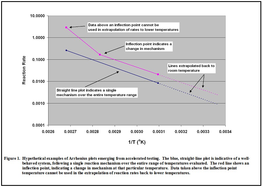
This plot also allows verification that a single mechanism operates over the range of temperatures evaluated. A single mechanism is a crucial requirement for temperature-based accelerated testing and any significant deviation from linearity or, more significantly, an inflection point, would indicate multiple mechanisms and would invalidate conclusions based on data obtained at temperatures above the linear part of the graph or above the inflection point. This is illustrated in Figure 1.
Calculating Reaction Rates at Different Temperatures:
Once the activation energy and modified pre-exponential factors have been obtained, the reaction rate (vT) can be calculated for other temperatures of interest, particularly at lower temperatures where the rates are too slow and take too long to measure empirically.
This is done using the logarithmic version of the Arrhenius equation.
First, calculate Ln(vT) as follows:
Ln(vT) = Ln(C’) – Ea/RT [7]
Then calculate vT:
vT = eLn(vT) [8]
where
vT = The reaction rate being calculated at Temperature (T) (mol L-1 s-1)
T = The temperature at which the rate is being calculated (K)
Ea = Activation energy of the reaction (J mol-1)
R = Universal gas constant (8.3143 J mol-1 K-1 )
e = Base of natural logarithms (2.71828)
C’ = Modified Pre-exponential factor (mol L-1 s-1)
Ln(C’) = Natural logarithm of the modified pre-exponential factor which is equal to the y-intercept of the Arrhenius plot
Time-to-Failure Analysis:
Accelerated testing is usually conducted by testing a device at different temperatures and monitoring the time elapsed until the device fails, based on some specified performance criteria. The measured time is the time-to-failure (TTF) for that device at each test temperature evaluated.
The reciprocal of the time-to-failure (1/TTF) gives an average rate of the reaction leading to failure (vT). It is this average reaction rate that is used in the Arrhenius analysis of the accelerated test data. The units of vT are s-1.
In most cases in accelerated testing applications, the exact reaction mechanism is unknown which means the order of the reaction and the actual reactant concentrations are also unknown.
Analysis of the data is done in the normal way by plotting the natural logarithm of the reaction rate (Ln(vT)) in s-1 versus 1/T (K) and determining the slope and y-intercept of the resulting line over the region where the line remains linear. Again, any deviation from linearity would indicate a change in mechanism.
The slope of the line would be equal to -Ea/R, from which the activation energy (Ea) can be readily obtained. The y-intercept would give the value of the modified pre-exponential factor (C’).
If the reaction mechanism is not known, which is usually the case in device time-to-failure tests, then the value of the y-intercept (C’) is interpreted to be the pseudo modified pre-exponential term having units of s-1.
To calculate the time-to-failure at different temperatures, first calculate the reaction rate (vT) at the temperature desired using the logarithmic form of the Arrhenius equation, as follows:
Ln(vT) = Ln(C’) – Ea/RT [9]
vT = eLn(vT) [10]
where
vT = The reaction rate being calculated at Temperature (T) (s-1)
T = The temperature at which the rate is being calculated (K)
Ea = Activation energy of the device failure reaction (J mol-1)
R = Universal gas constant (8.3143 J mol-1 K-1 )
e = Base of natural logarithms (2.71828)
C’ = Pseudo modified pre-exponential factor (s-1)
Ln(C’) = Natural logarithm of the pseudo modified pre-exponential factor which is equal to the y-intercept of the Arrhenius plot
Next, calculate the time-to-failure in seconds by calculating the reciprocal of (vT). Convert the result to different time units (e.g. days, weeks, months, or years), as follows:
Time-to-Failure (TTF) (sec) = 1/vT [11]
Days = TTF / (3600 * 24) [12]
Weeks = TTF / (3600 * 24 * 7) [13]
Months = TTF / (3600 * 24 * 30) [14]
Years = TTF / (3600 * 24 * 365) [15]
A Useful Approximation:
For chemical reactions, the general rule of thumb is that the reaction rate will double for each 10C rise in temperature. In this case, the time to failure (TTF) at some temperature (T2) can be estimated from the time to failure measured at a different temperature (T1) using the following equation.
TTF T2 = TTF T1 * 2((T1-T2)/10) [16]
When TTF values are expressed in seconds and Equation 16 is plotted as Ln(1/TTFT2) versus 1/T (K), a straight line is obtained having a slope of -7,545.6, which equates to an activation energy (Ea) of 62,736.4 J mol-1. The Y-intercept value will vary, depending on the value of TTFT1 selected. Note that 1/TTFT2 gives the reaction rate in sec-1 from time-to-failure data where TTFT2 is expressed in seconds.
This “rule of thumb” relationship is often used when empirical test data are not available or are insufficient for a complete Arrhenius analysis. For example, if the time to failure is known at one temperature, 70C for instance, the time-to-failure can then be estimated at other temperatures.
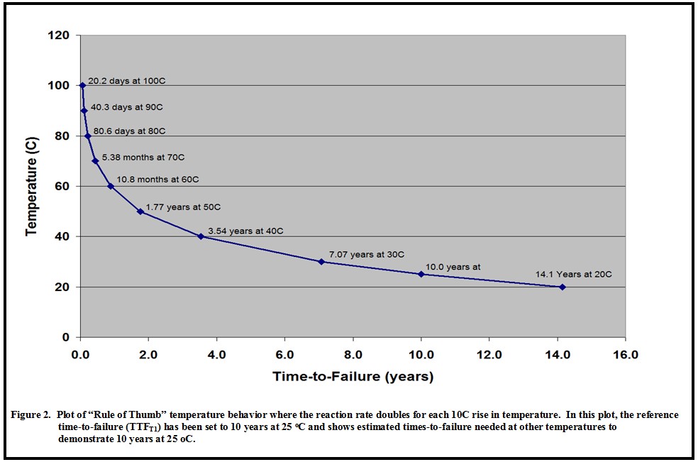
Equation 16 is also useful to estimate test times needed to demonstrate a desired product life. For example, as shown in Figure 2, to demonstrate a 10-year shelf life at 25C, the product would need to survive for at least 3.54 years at 40C, 1.77 years at 50C, 10.6 months at 60C, 5.38 months at 70C, and 80.6 days at 80C. This information allows one to set up a well-designed test program to get the data needed for a full Arrhenius analysis. It also allows development programs to be properly designed to ensure that enough time is allocated to do the testing needed to achieve and demonstrate the required product life.
Wrapping Up:
Accelerated test methods are an important part of our technology development in the modern era.
To develop and market robust products, manufactures must know how long their products last under a wide range of conditions and optimize their products to give the longest life possible.
Temperature-accelerated testing methods are crucial to achieving those goals.
Initial testing should be conducted over a wide temperature range to provide enough data points for a statistically significant regression analysis to establish the activation energy and modified pre-exponential factor for the system being studied.
Initial testing should also typically be conducted at temperatures high enough to establish the upper temperature limit for the system. That is, the temperature where additional failure mechanisms are initiated. Knowing this temperature limit is important because, in product development and quality control testing, rapid turnaround of the test results is a great advantage, and the higher the temperature, the shorter the test time. But one must be careful to only test in the linear region of the Arrhenius regression line, so it is important to know where the deviation from linearity occurs.
For chemical systems, such as batteries, the upper temperature limit is often in the region between 70C and 100C while for semiconductor and other solid-state devices, it can be 130C or higher. The upper temperature limit, as well as the activation energy and pre-exponential factor are critical parameters for manufacturers to know for each of their products.
Temperature-accelerated testing methods are powerful and scientifically sound. Every manufacturer should use them to deliver the best possible products to their customers.